3.3 Sub synth amp map
The questions that initially stimulated the next study piece had a focus on how digital sound might be made visible on screen; in practice, however, the pertinent questions soon become of how that sound is being made in the context of its visual representation on screen.
To introduce sub synth amp map there follows a brief discussion contextualising my work in relation to the practice of live coding. The sub synth amp map work is then described with further context. As with visyn, this piece demonstrates how aesthetic concerns have been explored and developed towards the formation of the more substantial pieces in the portfolio.
3.3.1 Live Coding with MaxMSP
Live coding 'has become so prominent as a practice within computer music' that it (almost) needs no introduction' (Thor Magnusson, 2011, p. 610).
My first contact with the idea of live coding (LC) occurred in contrast to the concept of live algorithms for music (LAM) in which I had interest during my MA studies (Freeman, 2007). Whereas LAM are conceived as independent software entities that may interact musically in an improvised performance setting with separate human players (Blackwell and Young, 2006; Bown et al., 2009), the LC paradigm is of humans creating improvised software structures during a performance. After at first viewing LC as a curiosity, the appeal of its aesthetic has gradually infiltrated my perspectives on computer music and software art. In my ongoing activities as a laptop-performer – leading up to and during this project, independently and as an ensemble performer – I have taken to embracing what I see as LC principles to varying degrees.
In practice, LC performances are framed by various a priori factors. Questioning some of these factors may help elucidate the unexpected role of LC in this project. The question I ask first is: at what level of abstraction is a coder coding? One may choose to begin by constructing the algorithms of sound synthesis, or (more typically) one may focus on generative algorithms that trigger and alter available sounds. Relatedly it can be asked: what is the programming environment of choice? Choosing to live code in a particular environment determines many aspects of the performance, and
the difficulties, or the near impossibility, of comparatively studying live coding environments due to the markedly different background of the participants and the diverse musical goals of the live coders themselves
have been discussed by Magnusson (2011, p. 615), who also writes that (p. 611):
Artists choose to work in languages that can deliver what they intend, but the inverse is also true, that during the process of learning a programming environment, it begins to condition how the artist thinks. […]
Learning a new programming language for musical creation involves personal adaptation on various fronts: the environment has an unfamiliar culture around it, the language has unique characteristics, and the assimilation process might change one's musical goals.
Chapter six (§6) will address some of these issues further in relation to the development of the sdfsys environment within MaxMSP which is my chosen environment for both live and compositional coding.
Common within, but not necessarily universal to, LC performance practice is to mirror of the performer's computer screen to a projector such that the audience may see what is happening in the software. By showing the screen in this way the audience have opportunity to visually engage with what the live coder is doing. The LC aesthetic thus offers an interesting perspective for this project, and its exploration of visual representation of sound. These are, again, matters to which the thesis will later return; in this chapter it is the use of MaxMSP as an LC environment that provides context to the sub synth amp map piece.
[n3.10] For example via http://livecoding.co.uk/doku.php/videos/maxmsp/about. My own contribution that collection, comprising sessions recorded between 2009 and 2011, is at http://livecoding.co.uk/doku.php/videos/maxmsp/sdf
Video examples of LC in MaxMSP can be found online.[n3.10] As an LC environment, when starting from an empty patch, MaxMSP lends itself to performances in which an 'instrument' of sorts is first created, and is then – while possibly being further added to or modified – played either with human or algorithmic (or both) control of parameters. Emphasis on the soundmaking aspect is in contrast to an event-making focus in LC environments that host ready-made instruments; Impromptu, for example, is an AudioUnit host (Sorensen and Gardner, 2010). The algorithmic control of traditional CMN-like concepts (such as pitch and rhythm patterns) tend to be prioritised in LC performances with Impromptu, although it is possible to write custom DSP algorithms in that environment. Heeding Magnusson's sentiment that comparative study of environments is near impossible, the preceding comparison is intended only to draw attention to where my aesthetic interests are situated: that is with soundmaking more than event-making. I am also attracted to the way that expressing musical ideas through code in real-time embraces nowness, and the general sense of transience that I perceive in LC aesthetics. There is the nowness of the moment within the duration of a performance, where the coder creates a musical macrostructure extemporaneously. Also – and in the context of computer programming as a practice that has existed for just a few centuries – there is a sense of nowness at the supra-scale of time of music (Roads, 2004, p. 3): in the history of human musicking, LC is very much a new phenomenon because it is only in recent decades that computers that are portable enough to carry to performance venues, with real-time audiovisual processing capabilities, have come to bear LC praxis.
3.3.2 From passing thoughts to pivotal theories
Work on sub synth amp map began as a live coding rehearsal exercise: the inception of this short study piece was as a first experiment toward an approach for the live coding of real-time audio synthesis with visualisations also live coded in MaxMSP. The improvised implementation uses similar visualisation techniques to those found in the visyn system, but here the system starts with an algorithm for sound synthesis, and then the output of that is taken both to be heard and seen (for further comparison of the two systems see §3.3.8 below).
From one perspective, the patches that comprise this piece are the result of passing thoughts manifest in code, designed and implemented on-the-fly and motivated by swiftness in generating output. However, given that the initial patch was saved – which is not always the case for live-coded practice pieces that are often allowed perish as fleeting moments – and that it was later returned to for further development, the patches may together be looked upon as rough sketches towards what may have, but did not (in of itself), become a much larger system. From another point of view these pondering prototypes illustrate a number of significant breakthroughs in my own understanding of the aesthetic principles and compositional processes guiding this project.
The creation of sub synth amp map was also, in part, a response to the following line of questioning: Keeping in mind some of the ways that physical aspects of sound have been seen to manifest as visual forms on various types of surface (§2.1) – and how when certain conditions are met within a physical system, visual manifestation of sound waves appears to be spontaneous and inevitable – are there any equivalently natural, or neutral, systems for manifesting 'digital sound' on screen? Rather than modelling, in software, the physical systems that give rise to visualisation of acoustic phenomena, can methods of representation be found that are somehow native to the screen? If so then such natively inevitable algorithms might well be approachable within LC contexts, for surely they would require little coaxing to manifest. Any methodology emergent in this vein is, of course, bound to be dependant upon the programming environment in which one is working. The visual direction of this piece was greatly influenced by the thought pattens that visyn had previously put into practice.
3.3.3 Names and numbers
[n3.11] Both here and in sdfphd_appendix_B_subsynthampmap.pdf, found within this work's folder of the portfolio.
[n3.12] As described by International Standard ISO 8601, see for example http://www.cl.cam.ac.uk/~mgk25/iso-time.html or http://xkcd.com/1179
Files associated with this study piece are located in the 'sub_synth_amp_map' folder of the portfolio directories. Discussion of this work[n3.11] is to be read in view of sub_synth_amp_map.maxpat which is an amalgamation of various patches that had each taken a slightly different approach to the same material. Within that folder it will also be seen that many of the maxpat and outputted audiovisual files carry in their filename the date on which this study piece was started (20100221). The naming of things by their date of creation is favoured because, to give one reason, it provides real-world meta-context to the content. It is the YYYYMMDD format[n3.12] that is used, and this is in contrast to the DDMMYYYY format employed, for example, by James Saunders in his modular composition #[unassigned] (Saunders, 2003).
In the case of this particular piece, edits and outputs that were made when returning to the work at a later date have retained the numeric name given to the original patch; although I am presenting this piece here with its four-worded title, the numerical 20100221 is considered an alternative title to the same work. The fact that audiovisual outputs created from this work on later dates are named with the numeric title date could cause confusion, which is why I have chosen to draw attention to the matter here.
3.3.4 Looking at sub synth amp map
The title, sub synth amp map, reflects the processes at play within the code of this piece, and was assigned to the work when a short video of the audio and matrix output was published online; eight examples of the matrix output, equivalent to still frames of the video, are shown in Figure 3.4 below. [click image to see the full-res .png; also, another eight examples, showing more variation in the typical output of the piece, are presented in Figure 3.9]
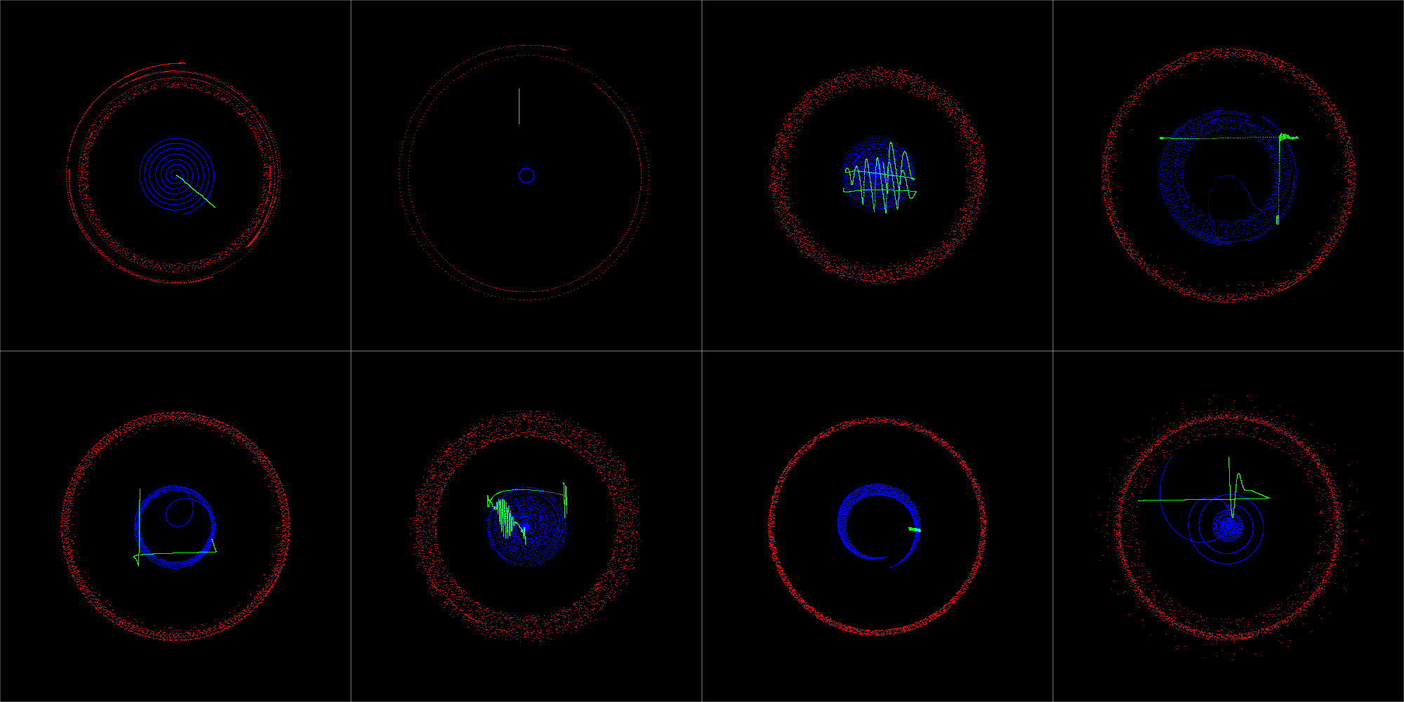
Figure 3.4: subsynthampmap_matrix_examples_4x2b.png
The 'sub synth' part of the title makes multiple references to the content of the piece: it refers to the subtractive synthesis method of soundmaking employed, and to the way that sub-sonic frequencies are used within that synthesis, both for modulation of the filter parameters, and in the audible input part of the synthesis (but the system is not limited to the using frequencies of the sub-sonic range). In the live coded design of the synthesis algorithm, a saw-tooth waveform was chosen as input to a low-pass filter with resonance; that waveform was chosen both because of its visual shape in the time-domain, and because it is harmonically rich in the frequency-domain. The sinusoidally modulated filtering of that input signal provides a time varying timbre that was quick to implement. When the saw~ oscillator object is set to very low frequencies, its audible output is similar to that of the twitching-speakers described (in §3.1.1) above: the sudden change in amplitude at the hypothetically vertical point in the saw-tooth waveform creates an impulse, or click, while the intermediary ramp period of the waveform is inaudible but visually perceptible at those frequencies. With the fluctuating cut-off and resonance settings of the lowres~ filter object, the sonic character of such clicks changes over time. Figure 3.5 shows the 'sub synth' algorithm of which there are two copies running in the patch. One copy is connected to the left, and the other to the right channel of the stereo output to the digital-analogue converter (DAC); these two signals are also used within the software as equivalent to those generated signals that were labelled 'X' and 'Y' in visyn.
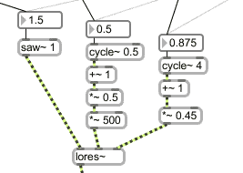
Figure 3.5: The 'sub synth' patch
[n3.15] Also see flow-charts in Figure 3.13 for comparison.
The 'amp map' part of the title refers to the way that the audio signals are 'amplified' before being 'mapped' to the dimensions of a Jitter matrix for display on screen; that is in contrast to the polar-cartesian conversions in visyn which occurred before value 'amplification'.[n3.15] Another interpretation of the second part of the title is simply that it is the amplitude of the input signals that are being mapped to matrix cell coordinate values. In sub synth amp map the angle values used in polar-cartesian stages translate to a great many revolutions of the circumference. Figure 3.6 shows the display mappings that were coded on-the-fly to make use of the RGB layers of jit.matrix m 4 char 500 500 so that three independent, monochromatic, visual forms can be simultaneously displayed.
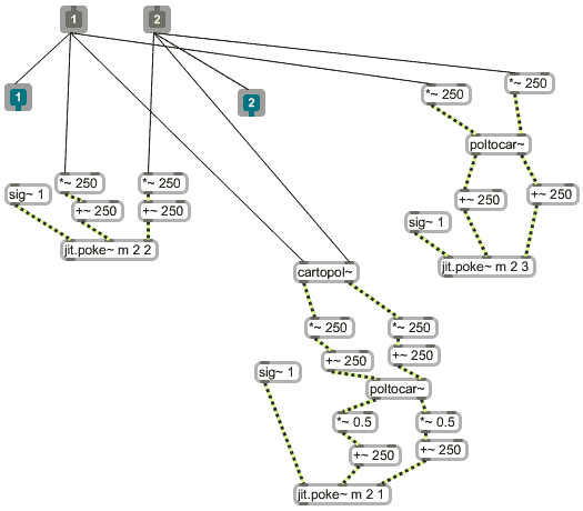
Figure 3.6: The 'amp map' patch
The grids of zero and one data values stored in jit.matrix m are visualised by a jit.pwindow object that has its size set to match the dimensions of the matrix so that each cell of that matrix will correspond to a pixel on screen. Default behaviour of the patch is for the matrix cell values to be cleared immediately ofter being put screen. An analogy, for this behaviour in the software, is taken from a conception of Cymatics (the Cymatic experience of seeing sound is of the movement present within a physical system at a given moment in time) by thinking of the input signals as acting to cause movement across the surface of the matrix. As real-time visualisation of sound, the attention of the sub synth amp map observer is brought to 'now' because the image of what has just happened is gone from view (almost) as soon as it appears. The rate at which the matrix is put on screen in the present system is determined by the metro 42 object (see Figure 3.7), which gives approximately 24 frames per second (fps). It is thus that the passage of time is brought into the visual representations of sound in the sub synth amp map system, and hence there is no need for time to be mapped to any other dimension of the display. If, as shown in Figure 3.7, the gate to the clear message is closed, then the traces will accumulate on the display. An example of this trace accumulation is shown in Figure 3.8 which is a matrix export saved to file during the initial coding session for this work.[n3.16]
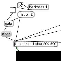
Figure 3.7: The 'matrix clear metro' patch
[n3.16] The file name '1' being given mindful of this being a first step towards my new way of working in software.
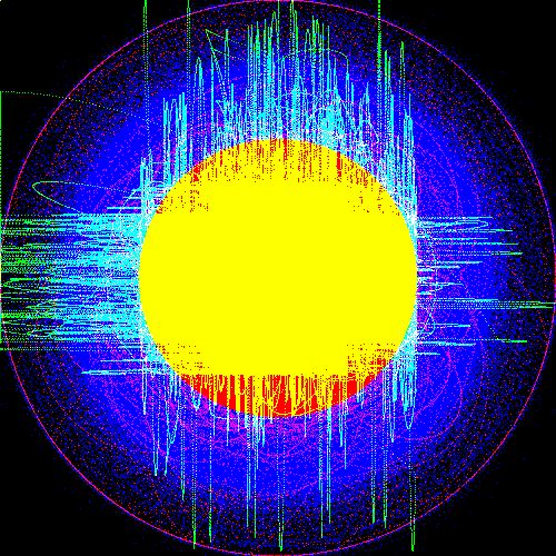
Figure 3.8: 1.jpg
3.3.5 Three layers, three mappings
Perhaps the most obvious method of mapping a pair of audio signals to dimensions of the screen pixel destined Jitter matrix is that of associating one signal with the x-axis and the other signal with the y-axis of the area on screen. In recognition of the commonality that such a mapping has in the use of oscilloscopes – which traditionally have a greenish phosphor trace display – plane 2 of the matrix is used as the target for this mapping which is also known as a vector-scope, goniometer, or phase-scope. The implemented algorithm for this mapping, as shown above in Figure 3.6, consists of three stages: (1) the two input signals, which have a range of -1 to 1, are first 'amplified' so that the range numerically matches the size of the matrix; (2) the signals are then offset so that the zero-crossing point of the inputs will appear in the middle of the display; (3) the signals are used to set the axis position values for the writing of a constant value (from sig~ 1) into the named matrix using jit.poke~ m 2 2 (where the first 2 is the number of 'dim' inputs, and second identifies the plane of the matrix to poke data to). Because of the way that matrix cells are numbered from the top-left corner of their two-dimensional representation on screen, if the two input audio signals happened to be identical (in-phase) then the display would be of a diagonal line from upper-left to lower-right corner. […]
The next mapping to be implemented was for the blue layer of the display in which the input signals, after being 'amplified' as in the green layer mapping, are treated as if they were polar-coordinates and processed by poltocar~; the derived cartesian coordinates, once offset to align the zero-crossing of the inputs with the middle of the display, then go to the jit.poke~ 2 3 object.
Lastly, the inverse translation of coordinate type (from polar to cartesian) is used for the red layer mapping. A process of trial and error lead to the configuration presented in the patch, which is a solution to the problem of polar coordinate values being unsuitable for direct connection to the cartesian-type 'dim' inputs of jit.poke~. The input audio signals are connected directly to cartopol~, the output of which is 'amplified' and offset in the same way as was the other two mappings. A second translation, back to cartesian, is then applied, and this is followed by a reduction in amplitude (to half the value range at that stage) and yet another offsetting stage before the signals go to jit.poke~ 2 1.
Figure 3.9 shows another eight examples of the sub synth amp map visual output.

Figure 3.9: subsynthampmap_matrix_examples_2x4.png
3.3.6 Input selections
A drop-down menu labelled 'Select source:' provides options for the choosing the input that will go to the display mappings sub-patch of the sub synth amp map patch. The last two options in the list allow arbitrary input of a two-channel sound source: either from the output of another active maxpat via adoutput~ – in which case, to prevent a feedback loop, the audio will not locally be connected to the DAC – or from a two-channel sound-file via sfplay~ 2 which has a playbar object for convenience. The other two source options in the menu select versions of the synthesised sound that was designed alongside the display mappings of the system. One of these, 'saw~lores~etc', connects to the real-time synthesis in the patch, while the other, '20100221_%i.aif' activates playback of sound-files that were recorded of a similar synth structure.
[n3.17] Video link, again: https://vimeo.com/9612972
With 'saw~lores~etc' selected as the source, there are three ways to control the sound which is mapped to the on screen display: (1) frequency values can be set using the number boxes; (2) these can be randomized within a narrow range by clicking the ; r bang message; or, (3) for a wider range of variety, there are 24 predefined presets which can either be triggered directly via the preset object or in a shuffled sequential order by clicks to the nearby button. These are the presets that were used in the video published in 2010,[n3.17] and – contrary to the sub-sonic frequencies rationale (§3.3.4) – include many higher frequency values.
When the '20100221_%i.aif' source is selected a continuous audio stream begins that is generatively formed from a set of sound-file recordings. There are 19 one-channel sound-files of duration ranging from a few seconds to a few minutes, and these were recorded during the initial LC rehearsal session as the idea to make more of this work began to set in. The simple algorithm for triggering this material is described by the flow-chart in Figure 3.10. There are two copies of this algorithm in the patch, in order to give two channels of audio. Because those two copies are opening files from the same pool of audio, and because the audio was all recorded using a particular range of parameter values, the 'stereo' sound that is heard and visualised contains a high degree of repetition, but the differing lengths of sound-file duration mean that the exact same combination of two sound-files at a given phase offset is unlikely to ever occur twice. The idea thus occurs again of things that are both ever-changing and always the same.
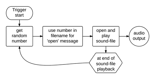
Figure 3.10: 20100221_sfplay_random_flow
3.3.7 Lamp-light, Laser beams, and Laptop screens
(3.3.7.a) Lissajous figures
Lissajous figures, the well known class of mathematical curves, can be made in the green layer of the sub synth amp map display when two sinusoidal signals – of frequencies that are harmonically related (by simple ratio) – are given as input via the 'adoutput~' source selection of the system. The four images in Figure 3.11 show some such examples: clockwise from top-left, these examples are formed of ratios 1:2 (an octave), 1:3, 2:5, and 1:4. These and other examples are discussed further, and with others, in sdfphd_appendix_B_subsynthampmap.pdf.
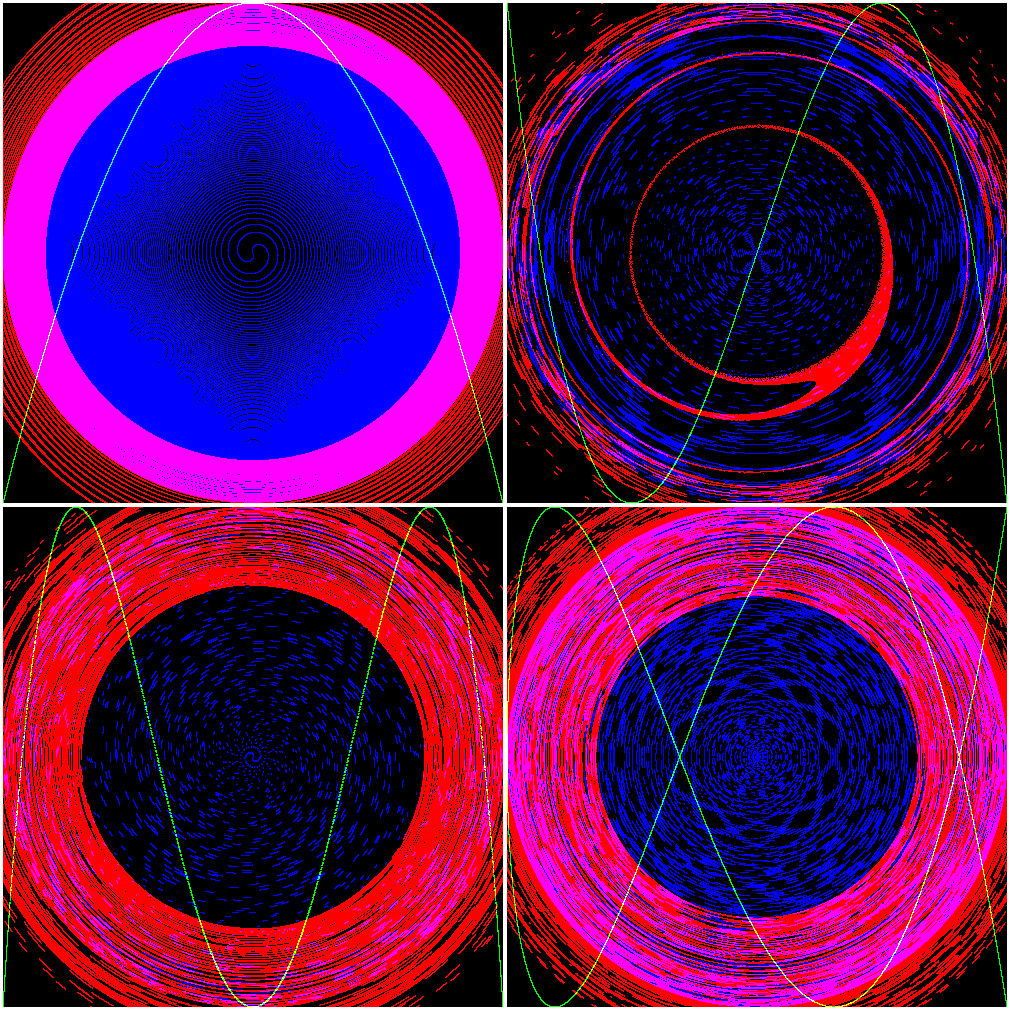
Figure 3.11: Four Lissajous
[n3.18] Illustrated in Plate VIII of that publication.
Lissajous figures are curves similar to those that are produced by the two pendulum harmonograph (Benham, in Newton, 1909, p. 29). The spiralling nature of harmonograms (see §2.1.3) is caused by the decaying amplitude of the oscillating pendulums. In sub synth amp map, the spiral formations are caused by the polar-cartesian conversions, and there is no decay of oscillator amplitude over time. A related visual effect of interference patterns, as seen within the blue and black area of figure the octave (top-left) in Figure 3.11 is also discussed by Benham who calls it 'the watered effect' (ibid. 1909, pp. 49–50):[n3.18]
By superimposing two unison figures that have been traced with a needle point on smoked glass, […] the result is that the watering is shown, while the actual spirals, as such, are not visible. […] Very beautiful effects may be obtained in this way, and if the two smoked glasses are mounted as lantern projections in one of the holders that allow for the rotation of one glass, a wonderful appearance is thrown on the screen, the watering completely changing form as the rotation proceeds.
(3.3.7.b) Lamp-light
Projected light is also what was used by Jules Lissajous in 1857: the curves that we know by his name were produced from:
the compounding of the vibrations of two tuning forks held at right angles. Mirrors affixed to the tuning forks received and reflected a beam of light, and the resultant curves were thus projected optically on a screen. (ibid. Newton, 1909, pp. 29–30)
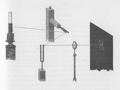
Figure 3.12: Lissajous mirrors
The described configuration of tuning forks, mirrors, a twice-reflected beam of light, and the projected figure manifest by these, are illustrated in Figure 3.12 (Ashton, 2003, p. 15).
(3.3.7.c) Laser beams
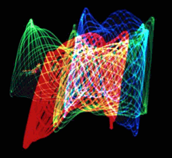
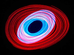
In 1968 Lowell Cross began a collaboration with Carson D. Jeffries to create a new system that employed those same principles of reflection. Working also with David Tudor, Cross established a method that used a number of laser beams – new technology at the time – each with a pair of mirror galvanometers controlled by amplified audio signals in place of the tuning forks, and 'the very first multi–color laser light show with x–y scanning [was presented] on the evening of 9 May 1969' (Cross, 2005). Three images from that Audio/Video/Laser collaboration are reproduced below:
[n3.19] Online at http://www.lowellcross.com/articles/avl/2a.Tudor.html [accessed 20130619]
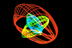
VIDEO/LASER II in deflection mode, image 1 of 3. Tudor: Untitled, © 1969.[n3.19]
[n3.20] Online at http://www.lowellcross.com/articles/avl/2b.VideoIIL.html [accessed 20130619]
VIDEO/LASER II in deflection mode, image 2 of 3. Cross: Video II (L). First photograph in deflection mode. © 1969.[n3.20]
[n3.21] Online at http://www.lowellcross.com/articles/avl/2c.Spirals.html [accessed 20130619]
VIDEO/LASER II in deflection mode, image 3 of 3. Jeffries: Spirals. © 1969.[n3.21]
[n3.22] Cited at second paragraph of §2
The periodic drive that was described by Collins (2012) – of artists returning to the 'acoustical reality of sound, and its quirky interaction with our sense of hearing' and to 'explore fundamental aspects of the physics and perception of sound'[n3.22] – seems to extend to the realm of visual perception while working with sound. Whether with lamp-light, laser beams, or backlit computer screen pixels, patterns such as those seen in sub synth amp map have historical precedence for being involved when human minds push toward new ideas by connecting with fundamental principles.
(3.3.7.d) Projected oscilloscopes
Before inventing the laser light show, Cross had already used other electrical equipment in a number of video pieces that also had focus on x-y scanning of the visual plane with audio signals as input; for example, here is an image from the 1965 work Video II (B):
[n3.23] Online at http://www.lowellcross.com/articles/avl/0x.VideoIIB.html [accessed 20130619]

Cross: Video II (B), © 1965.[n3.23]
[n3.24] There is also precedence dating to the late nineteenth-century for the 3D presentation of similar curve traces; the cited 1909 publication edited by Newton includes a number of stereoscopic harmonograms (Plate VI and Plate VII).
Recent works by Daniel Iglesia have also embraced the x-y 'oscilloscope' technique, but Iglesia has added a z-axis and the use of 3D anaglyph video projections;[n3.24] Iglesia describes his 2010 'work for two piano, two electronic percussion, and live video for 3D', Cardinality Aleph Two (Iglesia, 2012)[sic]:
This concert work is built an evolving AV system based on oscilloscopes. Here, each "orb" is created by three oscillators or samplers. The audio output of each becomes drawn coordinates in spacel the first maps to the X dimension, second to Y, and third to Z. This is the most literal and low-level possible mapping of sound and video.
(image: Iglesia, 2010)
(3.3.7.e) Laptop screens
In 2011 the Princeton Laptop Orchestra (PLOrk) premiered 24 Axes, by Iglesia, 'for 8 piece laptop ensemble, with live 3D video' (Iglesia, 2012)[sic, but italics added]:
24 Axes builds upon the composer's [3D oscilloscope], in which the performer controlled three audio signals […]. Via the relative frequencies and shapes of the three signals, various forms take shape. These shapes are the literal representations of the sound, nothing more.
For this scored ensemble version, each of the eight performers controls his/her own 3D oscilloscope. They follow a score that is being broadcast in real time to each laptop screen, with symbolic performance data traveling towards the performer in 3D space.
(image: Iglesia, 2011)
[n3.25] http://helopg.co.uk
Having arrived at 24 Axes, an ensemble work composed for PLOrk, the discussion of sub synth amp map has, in a way, come full circle: my study here began in the context of LC rehearsal, and much of my LC practice has been in the context of ensemble laptop performance, particularly with the Huddersfield Experimental Laptop Orchestra postgraduate group (HELOpg).[n3.25] In these contemporaneous works by Iglesia the audience is presented with 'literal representations of the sound' that is being produced. It seems to me that these works manifest from much the same intention as did the laser light shows by Cross et al. some 50 years earlier. Cross writes (1981) that his experiments with oscilloscope type display in performance of electronic music, that began in the mid 1960s, were in response to the abstraction of sound production from visual domain which Cross considered a problem in performance situations. When my development of sub synth amp map began – prior to reading of the contextualisation that has been given here – it was in mind that an audience may observe the programmatic process of mapping sound signals as well as the visual output of those mappings.
There seems to be an inherent propensity of studied sound to manifest visually as orthogonally projected oscillations. Such mappings can be applied both to analytical ends (as in the studies undertaken by Lissajous, and in the stereo phase-scopes used today by audio engineers), and to aesthetic ends (as in those systems developed by Cross, and by Iglesia). Arising from my own interest in polar coordinate systems, and their possible applications in computer music software, sub synth amp map has also integrated polar-cartesian transformations while mapping signals, and the results have been influential towards subsequent works within the project. For this project, however, the main point of interest arising from the study here is as follows: when one composes music in conjunction with a direct mapping of sound signals to visual space, the organisation and control of soundmaking parameters in the music happens according to an aesthetic interaction with those visual representations.
3.3.8 Connections and comparisons between study pieces
As stated in §3.3.2 the data matrix techniques exhibited in the sub synth amp map study are similar to those found in the visyn system; comparison of these two systems is aided by the overview flow-chart representations shown in Figure 3.13: in visyn the data that is displayed visually occurs with the flow-chart prior to the audio signals that are heard from the DAC; the sub synth amp map system reverses that flow in the way that the audio signals connected to the DAC occur before the displayed data.
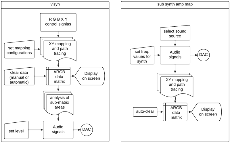
Figure 3.13: Visyn and sub synth amp map flow
My work often progresses by looking for ways in which elements of a system can be reversed. Another example of elements switching roles is shown in a comparison that looks ahead to the piece that is discussed in the next section. In the flow-charts of Figure 3.14, below, data writing poke operations implemented in two works are illustrated; sub synth amp map can be typified as system in which audio inputs are mapped for continuous control of to which cell of matrix a constant data value will written. In contrast, the model of a gramophone has that relationship inverted: audio input continuously changes the data value that is to be written while a consistent algorithm (the model abstraction) controls to which cell that data is written.
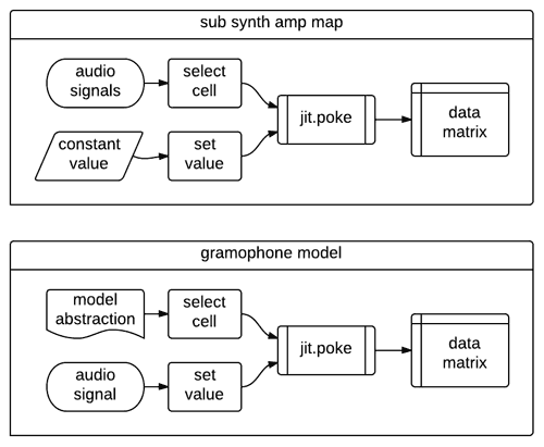
Figure 3.14: Comparative poke flow
In conclusion to this section a different connection is made: the Jitter matrix to which RGB traces are drawn in the visyn system is processed by the jit.wake object in order to 'soften the edges' of the otherwise 'pixelated' curves. The visual effect being aimed for was that of a glowing luminescence, and the comparison to the images by Cross of VIDEO/LASER II in deflection mode (see §3.3.7.c) can now be made. The slow fading that the wake effect in visyn causes of the visual traces is also manifest (albeit subtly) in the sounding of that system. It is noted now, however, that the visibility of pixel corners in the cell-quantized representations of theoretically continuous curves is something that is now celebrated in the on screen software medium within my work.