3.4 Conceptual model of a gramophone
As a composer seeking new methods for organising sound, I have sought to construct ways of understanding the things-with-which-I-work by bringing my attention to the mundane and mostly taken-for-granted aspects of those things. In the preceding sections of this chapter, that approach has been mostly applied to the computer screen and the use of its pixels; in this section it is the very existence of recorded sound that is questioned. Continuing the theme of rethinking musical technologies that originate in the nineteenth-century, a conceptual model of a gramophone is the subject of the next study piece and which, then, becomes the basis for a software mediated composition (§3.5). Always with my questioning the goal is to inform and inspire both the creation of new systems for soundmaking and the making of music with such systems.
Historically, it was the phonautograph that introduced the recording of sound waves to a surface medium via acoustically-coupled stylus, and the phonograph then introduced playback of similarly captured sound, but it was the gramophone that introduced the use of disc surfaces, inscribed with a spiralling trace (groove), as a sound recording medium; the basic format of which is still in use today.
3.4.1 Analysis of motion
A brief analysis of the motion found within a gramophone is conducted toward construction of a conceptual model. In the archetypical gramophone playback system, one can think of there being three dimensions of movement: (1) there is the angular rotation of the disc, (2) the radial sweep – from outer edge toward the centre – of the stylus-head transducer, and (3) the motion of the stylus needle itself as it follows the contours of the groove that comprise the sound recording. It is not conceptually relevant to think about how those contour tracing motions of the stylus needle eventually reach human ears as sound: it is enough to think of the stylus as being connected (somehow) to the output of the playback system. Focus remains, for now, with those three dimensions of motion identified. Mechanically, the only active part of the gramophone system described is the turning of the disc for the angular rotation of the disc. The spiral cut of the groove naturally brings the other two dimensions of motion into being as the needle of the stylus head rests within the groove while the surface rotates. An alternative method for reading a gramophone disc is to let the disc surface be unmoving, and have the stylus head instead be mounted in the chassis of a forwardly active vehicle; thus is the device – pictured in Figure 3.15 (Sullivan, 2005) – that is sold under the name Vinyl Killer (Razy Works, 2008):
Vinyl Killer is a portable record player […] Instead of spinning your record, it coasts on the surface of the vinyl, gliding the needle over and into the grooves, churning out music from its own built-in speaker.
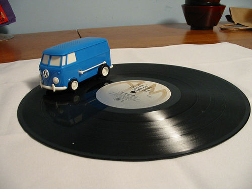
Figure 3.15: Vinyl Killer
When deciding to build a model of a gramophone it was with the idea that a Jitter matrix would act as the disc surface (albeit as a square, instead of a round, plane), and that that surface would not need to spin (rotation of a Jitter matrix is possible, but unnecessary here); instead the model would include an active stylus head that moves around the on the surface. My model is described as a conceptual one; this study is not an exercise in physical-modelling. With a conceptual model the actual physics of reality need not be of concern, only the idea of the thing in question need be taken as the basis for reconstruction of that thing in another domain.
[n3.26] details online at http://dorkbotsheffield.lurk.org/dorkbotsheffield-1
[n3.27] One may speculate, however, that as some who was born in 1984 I may be of one of the last generations to have grown up with vinyl records as the mainstay of a music collection in the home. The gramophone-like disc format prevails as a medium but it is no longer dominant in the domestic environment.
The work being described here was presented with a similar narrative in June, 2011, at the DorkBotSheffield event.[n3.26] Within that presentation, and here too, the ambiguity that has, by this stage, crept in to the discussion with regard to what exactly is being referred to by a 'gramophone', is not of great concern: the ubiquitous influence of such systems within our culture puts the subject matter well within audiences' consciousness.[n3.27] Nevertheless, the model deserves a definite basis, and so the question is posed 'what, in essence, is a gramophone?', and then the answer given (in a form inspired by Senryu poetry) as a 17-syllable stanza:
		a gramophone is
		a spiral track of sound-waves
		on a flat surface
Upon that concise abstract the conceptual model is based. For implementation of the model in software, the surface aspect of the gramophone – as mentioned above – can be a Jitter matrix (a plane of float32 data type is used), the sound-waves can be obtained from the computer's analogue-digital converter (ADC), and the spiral track can be defined by a curve drawing algorithm.
3.4.2 A spiral on the surface of a plane
To be in keeping with the above analysis of motion in a gramophone system, temporal navigation of the spiral curve that represents the groove should be the consequence of only one 'active drive'. The theta value input to the Archimedean spiral equation provides that behaviour: the polar equation to draw the Archimedean spiral is (Weisstein, 2003):
r = a · (theta)
To understand that equation in terms of data-flow, it can be read from right-to-left: the angle value theta is the input that is processed by multiplication with a to give the output r. The range of the theta input is taken to be from zero to infinity, and the curve, too, is theoretically infinite in its expansion.
Most of us are far more accustomed to working with and thinking in cartesian-type spaces, and although polar-coordinate systems are easy enough to understand, they can be confusing in practice; not least because software implementations of them can differ greatly in terms of what angle appears where on the round, and in what unit of measurement. The visual direction by which angle values will increase can vary too: clockwise motion may represent positive or negative change. It is also common, in some disciplines, for the radius value to be referred to as amplitude, but given the commonly applied usage of that word in relation to sound I prefer to remain with the term radius in the context of polar-coordinates.
Frequent return to polar-coordinate representations in my work is related, for instance, to the perception motivating this project that the rectilinear conception of sound confines musical thinking, and that a more circular conception of things may lead to different compositional decisions being made. There is also the existence of visual 'form constants' which are innate to the human visual cortex (Wees, 1992; Bressloff et al., 2002; Grierson, 2008; Bókkon and Salari, 2012), and are geometrical patterns that can best be described in polar-coordinate terms.
Where an Archimedean spiral represents a gramophone groove, the theta value represents the linear time-domain of the recorded sound. The value of a, in the Archimedean spiral equation, serves to determine both the direction of the spiralling (rotation is clockwise when a < 0) and the size of the spacing occurrent between successive rotations of the line. For every 360 degrees (or 2π radians) increase in theta the radius will increase by the same specific amount.
More recently invented disc shaped storage media start their tracks (of digital data) toward the centre of the disc and spiral outward, and this is also the way of the Archimedean spiral: increasing the theta value is to move along the curve and radially away from the polar origin. In contrast, however, the time-domain groove of a gramophone disc begins from the outer edge and progresses inward. It was therefore part of the implementation of my conceptual model that the appropriate inversion of values be made within the algorithms so that increasing time would provide a decreasing theta value over the required range. In order to reduce complexity for discussion, that aspect of the model is mostly absent in the following descriptions of the work.
3.4.3 Stylus abstraction
Before the model can be used to playback sounds, it must first be made to record them. The key to each of these processes is the stylus part of the system. An algorithmic representation of a stylus head has been constructed.
The 'active drive' of the stylus abstraction is a DSP sample-rate counter. When triggered to start, the counter value is processed with three parameter values that have been provided as input to the abstraction; the output is a pair of signals that provide cartesian coordinates for use with objects that access data stored as Jitter matrices. A flow-chart representation of the stylus abstraction is shown in Figure 3.16.
[n3.28] The flow chart illustration, and this document in general, use underscore notation for these parameter names (i.e. g_dur), whereas the maxpat uses a dash (g-dur); this discrepancy is indicative of a change in style within my programming during the project. While the MaxMSP interpretation 'g-dur' is as a single symbol, other languages might see it as '“g” minus “dur”' and so it would not work there as a variable name.
The 'Re-Trigger Mode' and 'Trigger Start' inputs are local to each instantiation of the abstraction. Values for the parameters that are named 'g_dur', 'g_mult', and 'g_a' [n3.28]are received the same to each stylus; this is so that the 'recording head' and the 'playback heads' – each with its own instance of the stylus abstraction – can be aligned to follow the same curve on the data surface.

Figure 3.16: Stylus abstraction flow
3.4.4 Gramophone_002_a
Files pertaining to this study piece are found in the 'model_of_a_gramophone' folder of the portfolio directories, and a neatened-up-for-presentation version of the first working prototype of the conceptual model is gramophone_002_a.maxpat. Construction of this model was a progression from the work undertaken in sub synth amp map, and many of the same principles are found here. There are three styli in the system, and these are represented visually on screen as red, green, and blue trace points of an RGB matrix. […] Figure 3.17 shows a flow-chart representation of the patch.

Figure 3.17: gramophone_002_a flow
Another version of the same patch, with '_i_o' appended to the file name, was cerated so that the system could be used within the context of a larger modular maxpat system within live performance; in that version of the gramophone model the ADC has been replaced by a receive~ object, and the DAC replaced by two send~ objects.
Two video demonstrations of the _002_a patch have been included in the same portfolio folder; the audio in these screencast recordings is from the output of the maxpat. The first of these examples is g002a_x1.mov (0 min 55 sec); during this video, microphone input is used to record human voice to the data surface […]. After input audio data has been written, the two read/playback-head styli are triggered – one, then the other – and the audio output can be heard. [When the] 'in-out-in' re-trigger mode is selected [(at c.39 seconds into the video, as shown in Figure 3.18)] on some of the inward passes of the spiral path, there must be a slight misalignment to the recorded data track because there a roughness to the sound reproduced which one can imagine as being caused by reading cells with zero data interlaced with the expected data. This glitch is caused by that the way the re-trigger modes have been implemented in this proof of concept prototype, but rather than looking upon it as an error or bug to fixed, the effect is embraced as having potential for creative exploitation; precise reproduction and high-fidelity are most certainly not the objectives here.
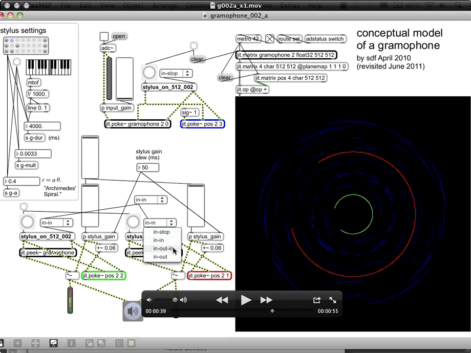
Figure 3.18: g002a_x1.mov (at 39 sec)
Running in the demonstrated way, the gramophone model can be thought of as a low-fidelity delay-line in which the effective sample-rate is variable across the period of the delay: there are less matrix cells per angular degree near the centre of the data surface than there are at the outer periods of the spiral curve. Whereas the whole of the data matrix is available, only those cells that are accessed by the stylus abstraction during the recording are actually used to store data. Although this may seem an inefficient use of system resources, contemporary computer systems are not short of memory space, and the method developed here has the aesthetic benefit of allowing the audio data to be displayed on screen in a very direct way, with very little intermediary processing: the matrix of float32 type audio data is simply copied to the 'blue' layer of a char type ARGB matrix that is added to the 'position matrix' of the same type (showing traces of the three styli) and is then put on screen (with cell-to-pixel correlation). Disadvantages of that simplicity are discussed below (§3.4.5).
The second video example, g002a_x2.mov (5 min 43 sec), resumes from where the first had left off, and continues with sound from a soprano melodica at the microphone input to ADC. For this demonstration, the pitch 'A-flat' was chosen to be played on the melodica because it has been found to manifest with a coherent six-armed pattern within some of the preset stylus settings that are used during the screencast video: see Figure 3.19. During the demonstration, the audiovisual output can be observed as audio data is written to the data surface and parameters of the patch are changed on screen.

Figure 3.19: g002a_x2.mov (at 3 min 16 sec)
When the stylus settings begin to be changed, at first only the duration value is reduced: playback continues over a smaller radius of the surface than before, but because the g_mult and g_a values are the same, the alignment of the reading curve is kept upon the written data track. As the g_a value is increased, so too is the radius of the spiral track and with that the data values being read to form the audio output signals are no longer being read in the same sequence that they were written. As long as the g_mult value is unchanged, however, the audio output retains much of the character of the original input.
The creative potential of the model, as it is implemented here, really begins to show when all three of the stylus settings parameters are altered, especially when taken to extremes. At 3 min 51 sec audio input is once again written to the data surface with the current stylus settings; the g_mult value is then altered and a pitch shift in the output can be heard. Soon thereafter all three parameter values are shifted through ranges that produce some delightful glitch textured sounds in conjunction with aliased and interlaced spiral patterns in the traces of the read-head paths (see, for example, in Figure 3.20).
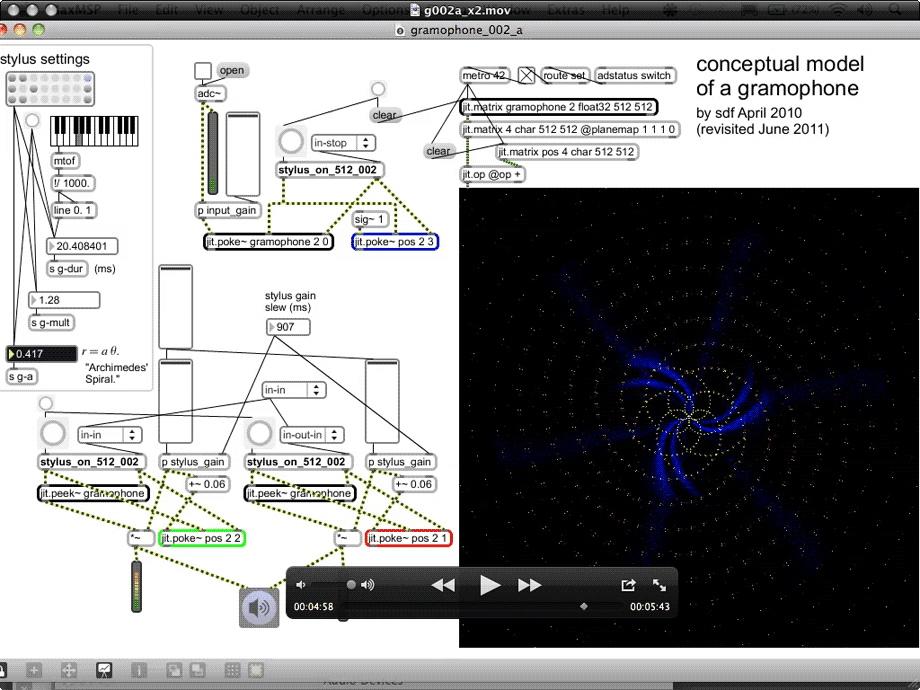
Figure 3.20: g002a_x2.mov (at 4 min 58 sec)
3.4.5 Interacting with _002_a: limitations and inspirations
[n3.29] But in works that are not included in the portfolio; see for example http://sdfphd.net/looking-at-sound/
Notice that in the blue layer of the display, the audio data appears as an intermittent trace that oscillates between blue and black. This use of blue on black was perhaps a poor choice for visibility of the data in general, but having green and red as representative of left and right had already been established in other works within the scope of this project.[n3.29] The method by which the recorded audio data is rendered here to the on screen display introduces truncation of the data values such that the visual representation includes only the positive values. Jitter automatically scales float32 values between 0 and 1 to the char data range of 0 to 255 that is used in the ARGB format for screen pixel colouration. The negative values of the sound recording are truncated by that mapping, and are thus represented visually the same as zero values. For a typical audio input recorded to the data surface there ought to be twice as many non-black cells shown on screen. It may also be considered that the non-linear perception of sound signal amplitude in human hearing perhaps ought to be a feature of the processes that convey audio data through colour level in a display. Representation of the bipolar data value range is something that the sdfsys development addresses (see §6.2.5). It was found unnecessary, however, to bring logarithmic scaling or similar into the methods for this aspect of the project.
Simultaneous observation of both the changes (on the RGB matrix display) and their causes is difficult, if not impossible, not only when watching back the example videos, but also when playing the patch itself. Visual manifestation of the three stylus abstraction control parameters as shapes on the data surface display is both spatially and conceptually removed from the interactive elements of the GUI on screen (the number boxes, sliders, menus, and buttons). One's attention is constantly split between two, or more, mental models of the system. My thoughts, at the time of creating this work and exploring its possibilities, thus became of how much better it would be to be able to keep one's eyes upon the shapes and impart control directly upon them within that space on screen; this concept I have come to refer to within my work as the 'integrated display' of audio and control data, and the sdfsys system was developed with that in mind.
Settings to which my explorations of the _002_a prototype soon habitually lead were of the short duration, great multiplication value type that produce a particular quality of audio output: as discussed further in §3.5.4, when the stylus abstraction path is set to such that the extremities of the curve are beyond the edges of the data surface fragmentation is introduced to the sound as the output signals oscillate with periods of data/no-data. To understand the clicks that may become buzzes in the resultant sound from these settings it is observed that the jit.peek~ objects, that are used to read values from the matrix cells, will always return zero when cells coordinates beyond those present in the matrix are requested. The data/no-data description is assuming that there is audio data within the matrix to be read during the periods of those such set paths that do cross the data surface.
Rather than developing the gramophone model patch toward a performance system – which may have included the addition of more read-head styli, more options for variety in their control, perhaps with a more integrated display – the work was instead steered toward a compositional outcome. Various intermediary stages of that development are omitted in favour of a detailed examination of the _005g version of the conceptual model of a gramophone.