4.3 Spiroid display of partials as arcs on an lcd in MaxMSP
In contrast to the FFT data displays described above (Rouzic, 2013; Storaasli, 1992), my own spiroid-frequency-space displays are based on the (more abstracted) data resultant from pitch tracking analyses; perhaps this choice of is approach can be linked to the above described genesis of the spiroid concept – with its initial focus on discrete pitches, rather than continua – but also it is a reflection of my interest in the perceptible cognition of aspects of sound: I chose to work with a smaller number of higher-level data, rather than with the hundreds of data points that an FFT provides. A double meaning is thus observed the description of a 'partial analysis' from pitch tracking, as contrasted to the more complete one of an FFT. The spiroid concept is also set apart from above given the examples of similar spirals by its application to the input of frequency value data (see §4.4), in addition to the output display of analysis.
This section describes my spiroidArc prototype, elements of which have been reused in a number of different works during the project. Construction of the prototype began in the run up to the official start of this project,[n4.12] and its development is a direct continuation of the incremental process described in §4.1.
[n4.12] With the conceptual and practical work progressing at various stages in the two year gap after my MA studies.
4.3.1 Analysis and display
Software implementation of the spiroid began with a visualisation of pitch analysis data from the fiddle~ object in MaxMSP;[n4.13] specifically, using the lists of frequency and amplitude values that describe the sinusoidal components, or partials, of the input audio. The amplitude value of each partial is used to set the (alpha) transparency of the arc representing that partial on screen (the greater the amplitude, the greater the opacity); the frequency values are converted to midi-pitch values from which the pitch-class and octave-level attributes are taken to determine the placement of the arc on the screen. The process is shown as a flowchart in Figure 4.11:
[n4.13] by Miller Puckette, MSP port by Ted Apel and David Zicarelli; available from http://crca.ucsd.edu/~tapel/software.html – my use of fiddle~ had continued despite the newer sigmund~ object being available.
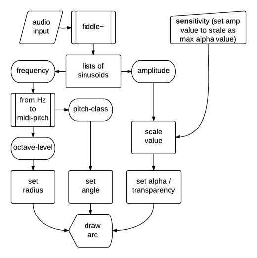
Figure 4.11: spiroid arc display flow
The lcd object has been used for drawing the arcs on screen, and the message format for doing that in a maxpat comprises the keyword 'framearc' followed by six numerical values that define the following three spatio-visual attributes:
- four numbers to define the square/rectangle bounds of a circle/oval (left, top, right, bottom);
- the starting angle of the arc (degrees, with zero at the top, ascending clockwise);
- the size of the arc (degrees).
In the spiroidArc patch, numbers for the square bounds of the circle to which an arc belongs are calculated by an abstraction[n4.14] which takes two inputs: a radius value (mapped, in this case, from the octave-level value of each partial), and a cartesian-coordinate for the centre point (fixed for this patch). The pitch-class value of each partial is multiplied by 30 to give the start angle in degrees, and the size of the arc is fixed at eight degrees (which is rounded up from 7.5 degrees which is a quarter of 30 degrees which is the angular size of a semitone).
[n4.14] The abstraction, originally named sqr.maxpat, was later renamed to ltrb.maxpat when it was upgraded to include patcherargs and pattr objects (c. November 2009).
It will be noted that the equations given in §4.1.4 are not explicitly present in the method described here; indeed the prototype described here was built prior to my formulation of those equations. The result, however, is the same: the radius increases at a constant rate as the frequency value is increased.
4.3.2 SpiroidArc
(4.3.2.a) a_demo_of_SpiroidArc300
The earliest example of my spiroidArc display that will be presented is spiroidArc300.maxpat; the number in the file name shows this was 'version three, revision zero' of the spiroidArc concept.[n4.15] […]
[n4.15] It was created, March 2010, en route to perform at Interlace #36, Goldsmiths (inclusive improv, 2010; Lexer, n.d.).
The following explanation is written of a_demo_of_spiroidArc300.maxpat from the spiroidArc300 folder in the chapter4 directory of the portfolio. There are some 'sound sources' in place for use as input to the spiroidArc patch that is embedded. When the demo patch is opened, it will look something like shown in Figure 4.12, but note that the 'zoom level' of the patch has been increased in this figure. The size of the display was intentionally kept small because it was designed to be on screen at the same time as many other GUI patches within a modular system. When the spiroidArc display is the only patch being used the zoom feature of MaxMSP can be used to increase the size on screen.
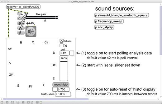
Figure 4.12: spiroidArc300demo1
The three sound source sub-patches are:
-
sinusoid_triangle_sawtooth_square
- the waveform oscillators, other than the sinusoidal, are antialiased; click on the graphic representation to switch between waveform shapes
- frequency is set by combination of three parameters (octave-level, pitch-class, fine-tune)
- panning is not in use: only right channel is output
-
frequency_sweep
- on/off toggle is master to toggles for both metro and gate~; in order to suspend the 'sweeping' of values, metro-toggle can be off while gate-toggle is on
- nslider (CMN stave) on the right can be clicked on; the one on the left is display only
- currently sounding pitch has its midi-name, midi-pitch number, and frequency Hz value displayed by objects in the patch
-
adc_sfplay
- using the input part of the standard Max IO utility patch
- left and right channels are summed
(4.3.2.b) Histogram of strongest pitch-classes
By implementing the spiroid curve to display the continuum from midi-pitch zero up there are several octaves of sub-sonic frequency values in the centre of the space. I decided to add a histogram of sorts that would draw radial lines, around the centre of the display, at the angles of the most present pitch-classes. A flow chart representation of the algorithm implemented for this is shown in Figure 4.13, and the histogram itself can be seen within Figure 4.14 (below) where the spectrum of a sawtooth waveform oscillator sounding at 65.406 Hz (midi-pitch 'C2') is displayed.
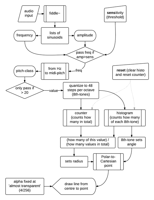
Figure 4.13: spiroidArc_histoFlow
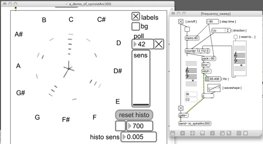
Figure 4.14: spiroidArc300demo2
(4.3.2.c) Background option to show 12TET angles
In addition to the optional 'labels' – which show the 12TET pitch-class names, and are toggled on by default – there is also a 'bg' option that will show the angles of the twelve equal divisions in the circle. Rather than just drawing radial lines at the twelve angles, however, I decided to use divisions of the colour spectrum to fill each sector (see Figure 4.15); I now consider this as a poor design decision, and the reasons for that are discussed below.
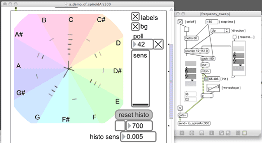
Figure 4.15: spiroidArc300demo3
4.3.3 Chroma paradox
(4.3.3.a) (chroma ≠ chroma)
The analogy of pitch-class as colour is compelling but in many ways misleading. This is a complex subject to approach, and the discussion here is worthy of further work; in the process of contextualising my aesthetic engagement with these matters I have been humbled by the potential scope of this subject, and can only present here the stage of exploration that I have reached. It is exciting to but glimpse for now the potential possibilities of seeking to unravel the chroma paradox.
What I now call the chroma paradox (described in §2.2.2) is something that arises from the full octave pitch-class-circle being commonly known as the 'chroma circle', which thus associates the angle attribute within a spatial representations of pitch- or frequency-space to colour; my suggestion is that this association is – if not paradoxical, then at least – contradictory to the consideration of morphophoric mediums and the respective (in)dispensability of colour and pitch, as outlined in §2.2.1. Clearly, this stance was arrived at only after the work of programming the spiroidArc display system described above.
Even within discussions of colour as colour, the word chroma can have different meanings depending on the context,[n4.16] and to some extent the same seems to be true of the word hue. In this work hue is understood as a dimension of the HSL (hue, saturation, lightness) colour-space: creation of the 12TET angle background seen in spiroidArc300 (Figure 4.15) was achieved by stepping at twelfth divisions of the hue value in the 'hsl' message to the swatch object in order to obtain the RGB values to use for drawing on an lcd. That part of the patch is shown in Figure 4.16.
[n4.16] For example, results at http://www.oxfordreference.com/search?&q=chroma – even without getting through the paywall of the web site – show definitions of chroma both as 'One of the three variables of colour (hue and value being the other two)', and as 'The quality or hue of a colour irrespective of the achromatic ( 1 ) black/ grey/white...' (accessed 20130924)
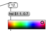
Figure 4.16: hsl_swatch
One premise of the analogy between pitch-class and hue rests upon the measurement of wavelengths and inter-domain application of the octave concept from sound to light – from acoustics to photonics(?) – for example Daryn Bond, describing implementations of the harmonic matrix, writes (Bond, 2011):
Colorizing the matrix makes use of the fact that the human eye sees somewhat less than one octave of light – from 390 to 750 nm [1][n4.17] In figure 10, the visible spectrum is ?artfully? extended from 373 to 746 nm. Pitch class is associated with a color, octave with brightness
[n4.17] [1] Cutnell, J. D.; Johnson, K.W. Physics. 7th ed. New York: Wiley, 2006.
The wavelengths of light beyond human perception are, in Bond's system, rendered as black; while this is a cunning compromise to one aspect of the chroma paradox, it does not help to remedy to ill-conceived situation of mapping pitch-class to hue in the spiroidArc. To get to the crux of this aesthetic crisis it is necessary to return to the subject of colour as an aspect of the medium being worked with.
The RGB colour-space has been discussed in chapter three (§3) because it is the method for defining colour values that is native to computer the screen medium. The RGB colour-space can be thought of in three-dimensional cartesian space as a cubic structure, as illustrated in Figure 4.17 (Otto, 2002); notice how the six colours used in the MoE pixels (§3.1) piece appear at the corners of this model.
Figure 4.17: RGB_cube
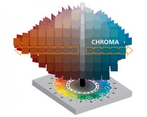
Many dictionary definitions for 'chroma' – particularly those that are, to me, the most convincing (cf. Colman, 2009) – make reference the 'Munsell colour system' which is named 'after Albert Henry Munsell (1858–1918)' (Colman, 2009), and 'is based on a three-dimensional model in which each color is comprised of three attributes of hue (color itself), value (lightness/darkness) and chroma (color saturation or brilliance)' (Munsell Color, n.d.). The Munsell colour system is thus closely related to the HSL colour-space, and when either of these is shown as manifest in three-dimensional space it is with a polar coordinate basis (Munsell Color, n.d.(text), and (image), n.d.):
The neutral colors are placed along a vertical line, called the ?neutral axis,? with black at the bottom, white at the top, and all grays in between. The different hues are displayed at various angles around the neutral axis. The chroma scale is perpendicular to the axis, increasing outward.
This amount of context is undoubtedly distracting from description of the spiroid, and yet – for the greater scheme – it is vital to bring mind to how the concept of colour is conceived of within the visual representation of aspects of sound.
(4.3.3.b) Double jeopardy
Not only is the chroma paradox casting heavy doubt on the use of colour described in §(4.3.2.c), but the assignment of the visual attribute of colour to aural attribute of pitch-class is also a superfluous doubling of visual attribute assignment: pitch-class equates to angle in the spiroid in a way that gains no benefit from a secondary identifier. The attribute of octave-level, however, would benefit from additional visual cues to help the viewer more easily perceive the relative radius values of the partials on display.
(4.3.3.c) Suggested remedy
The better choice for use of the hue scale within a spiroid-frequency-space display would be to have its continuum mapped along the frequency-domain continuum curve. I sketched this solution in February 2011, as shown in Figure 4.18, using just the additive primaries red, green, and blue to imply the colour continuum. It is noted that the Photosounder SpiralCM uses colour in precisely this way.
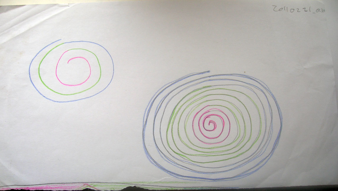
Figure 4.18: 20110221_0230